Predicting Stock-Market Behavior with Markov Chains
Apr 19, 2022
- Introduction
- What is a Markov chain?
- Types of Markov Chains
- Applications into Finance
- Creating a Transition Matrix
- Conclusion
Note: This was a mini-research project for a class called Machine Learning in Finance. It was taught by an amazing professor, Derek Snow, you check out his website here
Introduction
As I was first looking into Markov chains, it reminded me when I was studying graph theory for my algorithms class. There are some concepts such as BFS and DFS which weren’t fully applicable to Markov chains, but other ideas such as adjacency matrixes basically summarized the math behind calculating the probabilities. Generally it was interesting to see past topics I’ve learned connect with each other.
What is a Markov chain?
In a brief summary, it’s a model that helps predict a sequence of events. Future events can be predicted based on a probability from the present. An example of a chain predicting the daily weather is shown below:
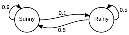
With this chain, we have two states: Sunny and Rainy. The next states from the starting states can understood as:
- If today is Sunny, there is a 90% it remains Sunny and 10% it becomes Rainy
- If today is Rainy, there is a 50% it remains Rainy and a 50% remains Sunny
Some interesting properties we can take note:
- The probabilities are also independent of past events, making the model technically “memoryless”. This is referred to as the Markov property
- The sum of a state’s next event probabilities will always equal 1. It doesn’t matter whether the chain is cyclic or not - Sunny: 0.9 + 0.1 = 1 - Rainy: 0.5 + 0.5 = 1
We can write some code to simulate the events over the course of a week:
# based from https://www.datacamp.com/community/tutorials/markov-chains-python-tutorial

import random
import numpy as np

states = ["Sunny", "Rainy"]
transitionName = [["SS", "SR"], ["RS", "RR"]]
transitionMatrix = [[0.9, 0.1], [0.5, 0.5]]

def activity_forecast(days):
    weather = "Sunny" # start with a sunny day
    for i in range(days):
        print(f"Condition: {weather}")
        if weather == "Sunny":
            change = np.random.choice(transitionName[0], replace=True,
            p=transitionMatrix[0])
            if change == "SS":
                weather = "Sunny"
            elif change == "SR":
                weather = "Rainy"
        elif weather == "Rainy":
            change = np.random.choice(transitionName[1], replace=True,
            p=transitionMatrix[1])
            if change == "RS":
                weather = "Sunny"
            elif change == "RR":
                weather = "Rainy"

activity_forecast(7)
Condition: Sunny
Condition: Sunny
Condition: Sunny
Condition: Sunny
Condition: Rainy
Condition: Sunny
Condition: Sunny
From the same image above, the Markov chain can also be represented as a probability matrix. This is where some linear algebra comes in handy:
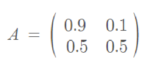
The odds of each state returning to it’s current state or switching can be described below. Another question naturally arises, how can we predict long-run probabilities? We can try modifying the code and running it for a longer period of time.
# Sunny = 1 since we're starting as Sunny
results = {
"Sunny": 1,
"Rainy": 0
}

def activity_forecast(days):
    weather = "Sunny" # start with a sunny day
    for i in range(days):
        # print(f"Condition: {weather}")
        if weather == "Sunny":
            change = np.random.choice(transitionName[0], replace=True,
            p=transitionMatrix[0])
            if change == "SS":
                weather = "Sunny"
            elif change == "SR":
                weather = "Rainy"
        elif weather == "Rainy":
            change = np.random.choice(transitionName[1], replace=True,
            p=transitionMatrix[1])
            if change == "RS":
                weather = "Sunny"
            elif change == "RR":
                weather = "Rainy"
        results[weather] += 1

days = 100000 # around 274 years
activity_forecast(days)
print(f"Sunny: {results['Sunny'] / days}")
print(f"Rainy: {results['Rainy'] / days}")
Sunny: 0.832332
Rainy: 0.167669
After a million iterations, we can see on average it’s sunny for 83.2% and rainy 16.8% of the time.
We can also use some linear algebra to calculate the probabilities for 20 days:
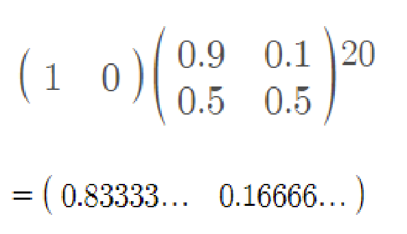
We can see the results are very close despite calculating for 20 days (more would require a lot of compute). If we are able to obtain an accurate probability matrix creating a Markov chain to see how markets move, it could be useful.
Types of Markov Chains
Let’s take a brief look at the two different types of Markov chains: discrete-time and continuous-time.
As their name applies, the two differ in how events transition to one and another. With the example above, we used a discrete-time Markov chain where a change in event happened within a day. There is a set interval for when changes occur. Examples of this could be examining market closing prices and determine whether it has gone up or down.
With continuous-time, the state is constantly changing. An example of this would be with a poisson distribution as the probability of events occuring constantly changes with time. This could be applied with day trading but would not be seemingly good as day trading can be extremely volatile. It would not follow the same Markov chain with it’s probabilities from day-to-day.
Now, how can we apply Markov chains to finance? What sort of states would there be? How can it be used?
Applications into Finance
A basic example of a Markov chain for the market condition is shown below:

This model has three states: Bull, Bear, and Stagnant markets:
- Bull Market: a period of time where prices are rising
- Bear Market: a period of time where prices are declining
- Stagnant Market: a period of time where prices are generally stable
Definitions of these types of markets may depend on different numerical values but are generally defined as changes of by 20%. With an accurate model predicting the state of the market, it would provide a good indicator whether or not to buy or sell.
Doing the above matrix calculations would return that:
- Bullish: 63%
- Bearish: 31%
- Stagnant: 5%
Generally when creating a model for finance, a discrete-time Markov chain would work better as changes to Bull/Bear/Stagnant markets do not happen frequently. Given that we can create a chain based on the type of market, the next question is how do we find those probabilities?
Creating a Transition Matrix
Using past historic data, is it possible to create a Markov chain that accurate reflects the market?
Through some Googling, the below is an implementation based off a blog post by Paranb Ghost. Some pseudo-code and the blog written by Manuel Amunategui applying Ghosh’s concepts into finance can also be found here
How do we classify the data?
Given previous market data, we have tons of information such as open and close prices. In Amunategui’s example, we’ll create a model that determines next-day volume up or down. We can choose different lengths of time to also potentially recognize patterns. For example:
2012-10-18 to 2012-11-21:
1417.26 -> 1428.39 -> 1394.53 -> 1377.51 -> Next Day Volume Up

2016-08-12 to 2016-08-22
2184.05 -> 2190.15 -> 2178.15 -> 2182.22 -> 2187.02 -> Next Day Volume Up

2014-04-04 to 2014-04-10
1865.09 -> 1845.04 -> Next Day Volume Down
Different patterns would help us indicate a trend. For example a repeated pattern of declines over the week would suggest a high probability that the next day would repeat the same pattern. We can take those types of patterns into account when building a model. Amunategui also mentions these patterns can be applied to other parts of financial data including market opens, highs, and lows.
Furthering down the classification, we can three different “groups” to classify how large of a percent change occurs between different days. The small group is “L”, medium group “M”, and large “H” corresponding to low, medium, and high. In the example below, Amunategui lists six changes and their classifications:
[-0.00061281019, -0.00285190466, 0.00266118835, 0.00232492640,
0.00530862595, 0.00512213970]

["M", "L", "M", "M", "H", "H"]
The groups can then be furthered combined into a “single event feature”. Taking a segment of four changes and chaining them together:
"HMLL" "MHHL" "LLLH" "HMMM" "HHHL" "HHHH" -> Volume Up
If you’ve noticed from the original classification into the low, medium, and high groups, there isn’t a way to differentiate between positive and negative trends. Following Ghosh’s approach, he actually creates two Markov chains: one for each.
In summary, we are taking patterns of market closes and opens, categorizing them into groups and sequencing them into two Markov chains: one for moves up and one for moves down. Using recent market data we can then use either chain to determine the probability for an increase or decrease.
Amunategui implements some functioning code here and it does give some decent results:
Confusion Matrix and Statistics
                Reference
    Prediction  0 1
                0 83 36
                1 110 98

        Accuracy : 0.5535
        95% CI : (0.4978, 0.6082)
        No Information Rate : 0.5902
        P-Value [Acc > NIR] : 0.9196

        Kappa : 0.1488
        Mcnemar's Test P-Value : 1.527e-09

        Sensitivity : 0.4301
        Specificity : 0.7313
        Pos Pred Value : 0.6975
        Neg Pred Value : 0.4712
        Prevalence : 0.5902
        Detection Rate : 0.2538
        Detection Prevalence : 0.3639
        Balanced Accuracy : 0.5807

        'Positive' Class : 0
As he states in the world of predicting stock market behavior, “anything over a flip-of-a-coin is potentially interesting”.
Conclusion
While Markov chains may not generally be the most popular tool in analyzing markets, it’s definitely a tool with broad applications. Ghosh’s methods of classifying the data is but one way of reducing features to build the model but other ways would most likely exist.
Though despite being a simple concept I learned in Algorithms, it was fun researching it’s application into something outside of computer science. I may have missed some details in the process and as well as the mathematics behind the model but it’s something that I will continue to learn.